1979–80
Neocognitron
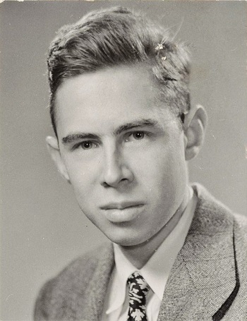
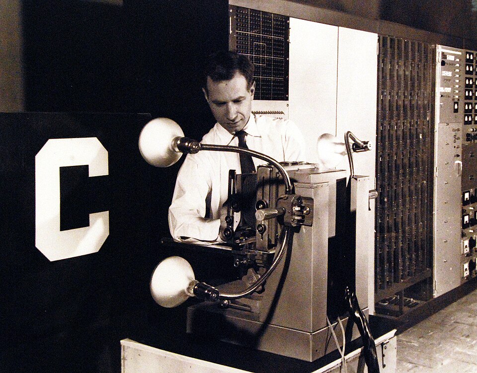
Kunihiko Fukushima builds a layered network of small, repeated feature detectors that inspired convolutional networks.
A SUMMARY OF OTHERS’ WORK
← Previous project: how a machine learns
Project write-up · NeurIPS 2012
In 2012 a neural network called AlexNet won an image-recognition contest by a margin nobody expected. Its recipe was not new. What was new was how it was computed: everything turned into vectors and matrices, so a graphics card could do millions of the same small calculation at once.
Start with step 1This is a summary, not original research. It follows the 2012 paper “ImageNet Classification with Deep Convolutional Neural Networks” by Alex Krizhevsky, Ilya Sutskever and Geoffrey Hinton, plus my own study notes. Everything interactive here was built to explain their work.
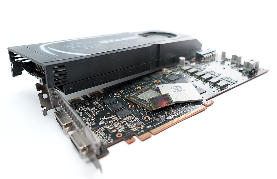
The recipe wasn’t new. What was new was the hardware: one big multiplication that a graphics card can run all at once.
On the last page a one-layer model scored a whole digit against one rigid template: W @ x. That is a dot product. This page asks what happens if the templates are small, slide across the picture, and are stacked in layers.
The question
Multiply pairs, add them up. That is a dot product.
A computer has no eyes. All it has is numbers. So the first question is a tiny one: how do you ask whether a small piece of a picture looks like something you are hunting for?
Try it below. On the left is a 3 × 3 snapshot. In the middle is a stencil of what you want: green squares mean “I want this bright”, red means “I want this dark”, blank means “I don’t care”. Multiply each square by the stencil and add it all up. It works like a shopping bill: every pixel is a line item, and the total is the match score.
In one line
A dot product multiplies matching pairs and adds them up. It is biggest when the snapshot looks like the stencil.
a · b = a1b1 + a2b2 + … + anbn
Finding it
One stencil, checked against every spot in the picture.
Step 1 compared one stencil with one small piece of a picture. But a real photo has thousands of pieces. So we do the same check at every spot, one after another, using the same stencil each time.
Think of the stencil as a set of expectations: “I expect dark on the left and light on the right.” At each spot we ask one question: do the real pixels here meet that expectation? The answer is a match score. Write every score into a grid, in the same position as the spot it came from, and you get a map of where the picture meets your expectation. For an edge stencil, that is a map of where the edges are.
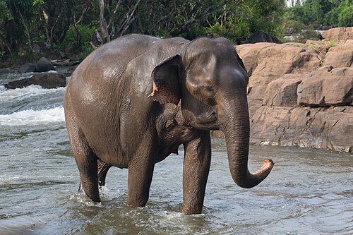
Below, you play the detective. Choose what you expect to see, then drag the magnifier over the elephant. Or press Scan and let it check everywhere.
In one line
One stencil, the same nine numbers, is compared with every spot in the picture. The grid of scores is a feature map: it shows where the picture meets your expectation. Doing this sliding check is called convolution.
map[i, j] = Σ K[u, v] · X[i + u, j + v]
Scale
Line the work up so thousands of workers can do it at once.
Checking 676 spots for one stencil is already 676 separate sums. AlexNet’s first layer checks 3,025 spots for each of 96 stencils, for every one of over a million photos, over and over. One worker doing one sum at a time would never finish.
A graphics card is more like a stadium of 512 workers who can all do the same simple job at the same moment. Race them below.
3ARace the Workers
3BLine the Work Up
There is a catch: the workers only help if their jobs are identical and lined up. So you rearrange the work first. Cut out every patch, flatten it into a row of numbers, and stack the rows into a table. Now each sum is one row times the stencil, and the whole table is a single multiplication. Making everything a list of numbers (a vector) and a stack of lists (a matrix) is called vectorization.
3CThe Same Trick for Text
It is also the idea behind ChatGPT. Words are chunked up, turned into vectors, stacked into a matrix, and operated on again and again (the biggest GPT-3 model repeats the step 96 times). AlexNet puts a label on an image; ChatGPT predicts the next word of a text.
In one line
Flatten every patch into a row, stack the rows, and one multiplication does every sum at once. In AlexNet’s first layer that is 3,025 rows, 96 stencils and 363 numbers per row.
Output (N × M) = P (N × k²C) × K (k²C × M)
Shape
A kernel for a colour picture is a stack: 11 × 11 × 3.
A colour image is three grids stacked: red, green and blue. Height × width × channels. A stack of matrices like that is called a tensor. A kernel for a colour image is a tensor too, and its depth must equal the depth of what it looks at. AlexNet's first layer uses 96 kernels of size 11 × 11 × 3.
Take the 11 × 11 × 3 chunk of the image under a kernel, multiply each kernel weight by the pixel value beneath it, and add everything up. That is 363 multiplications and one number out. A kernel has 363 numbers it can set freely, its degrees of freedom, and training chooses them. Each kernel is one more way of looking: the more of them, the more the layer can notice.
4ACount What a Kernel Sees
4BWhat Do the First-Layer Kernels Look Like?
The paper shows the 96 kernels its first layer learned. Some are stripes: edge and angle detectors. Some are checkerboards, which respond to fine texture. Some are colourful blobs, which say “green on this side, pink on the other.” The grid below is not the learned weights. I generated kernels in the same three families so you can see what each kind finds in a real photo.
In one line
A colour kernel is a stack as deep as its input, and the output size follows from four numbers. AlexNet’s first layer is (227 − 11) / 4 + 1 = 55; the paper says 224, which does not divide evenly.
⌊(n + 2p − k) / s⌋ + 1
Depth
The output of one layer is the input of the next.

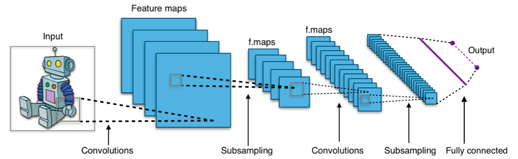
After the first layer you are left with 96 maps. They become the input of the next layer, whose kernels take dot products over those maps. The output of each step is the input of the next, so by the end every image has passed through a vast number of multiplications. AlexNet has five convolutional layers, then three fully connected layers that look at everything at once.
Where do the numbers go? Click a layer. A surprising split appears: almost all of the computation happens in the convolutional layers, but almost all of the weights sit in the fully connected ones.
In one line
Each layer’s output is the next layer’s input. Convolution does most of the arithmetic (92%), while the fully connected layers hold most of the weights (96%).
60,965,224 weights
724,406,816 multiplications
Learning
Training changes the weights, never the operations.
The operations inside AlexNet never change: dot products, a rectifier, pooling. Training changes only the weights those operations use. Backpropagation works out, for every single weight, which direction to nudge it so the answer is a little less wrong, by passing the error backwards through the layers.
On the last page the nudge was a flat plus or minus the picture. Here it is the slope of the error: w ← w − ε · ∂L/∂w. Below, a tiny network starts with random kernels and has to learn to tell vertical lines from horizontal ones. Nobody tells it what an edge detector looks like.
6AWatch a Kernel Learn
6BThe Paper’s Update Rule
AlexNet used a slightly richer version of that nudge. It keeps a running momentum so steps build speed in a consistent direction, and a little weight decay that pulls weights gently towards zero. The authors found the decay was not just a regulariser: it lowered the training error. Change the three knobs and watch a weight roll down a valley.
6CLearning, Seen in Weight Space
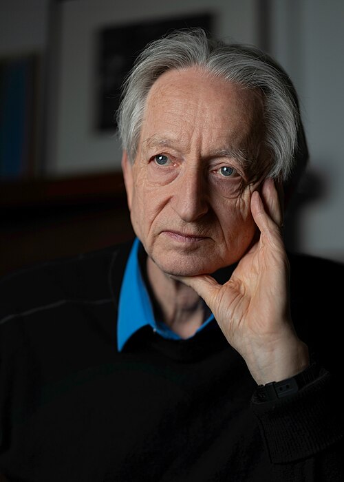
There is a picture that makes training click. Forget the image for a moment and treat the weights themselves as a point. A kernel with three weights is one point in 3D space; AlexNet is one point in a space with 60 million directions. Each training example puts a flat wall through the origin: weights on one side get it right, weights on the other get it wrong. Where every example’s right-hand side overlaps is a cone of feasible solutions. Training is just moving the point until it is inside the cone. Geoffrey Hinton draws exactly this picture when he teaches the perceptron.
In one line
Training never changes the operations, only the weights. Each weight is nudged against its slope, with momentum and a pinch of weight decay.
v ← 0.9v − 0.0005εw − ε·∂L/∂w
w ← w + v
The paper
Every section of the paper, in plain English.
The authors credit their result to a short list of choices, which they sort by importance in Section 3. Here is the paper in plain English, one section at a time. Each one has something to try.

In one line
The paper credits a short list of choices: ReLU neurons, two GPUs, normalisation and overlapping pooling, then augmentation and dropout against overfitting.
top-5 error
26.2% → 15.3%
Meaning
Distance in a learned space follows content, not pixels.
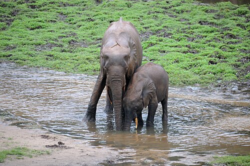
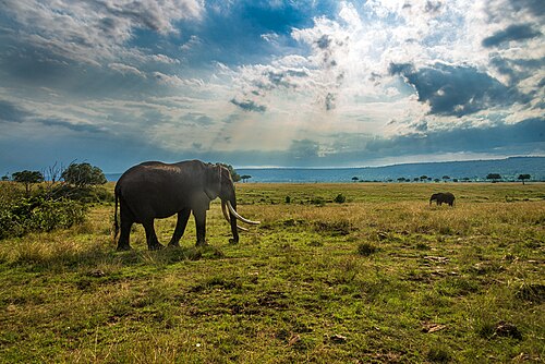
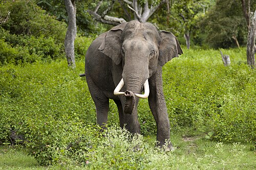
Every image the network sees is mapped through those levels of multiplications into a long list of numbers. Stop one layer early and grab it: a vector with 4,096 numbers. A vector is a point in 4,096-dimensional space. Just as you can measure the distance between two points on a map, you can measure it in that space.
The authors did exactly that. They took a test image’s vector, found the training images whose vectors were closest, and the nearest images were, for example, all elephants. Yet they note that at the pixel level those pictures are generally not close, because the elephants appear in a variety of poses. This is an embedding space: distance and direction mean something about the content, not just the colours.
8AElephants in Pixel Space
8BA Small Embedding You Can Explore
I can’t run AlexNet itself in a web page, but the digit model from the last page is a very small embedding. Its ten learned templates are ten directions, and a digit’s score for each is how far it lies along that direction. Pick two directions and every digit becomes a point on a map.
8CPicking the Closest One
Now the last step. When a new picture comes in, the network turns it into its vector, which is a single point. Every picture it has seen before is already a point in the same space. To recognise the new one, find the points nearest to it and let them vote. If most of the closest points are elephants, it is probably an elephant.
In one line
Compare two images by the distance between their 4,096-number vectors, not their pixels. Close in that space means similar in content.
d(a, b) = √( Σ (ai − bi)² )
Timing
An old idea, waiting for new hardware.
Almost none of AlexNet's ingredients were new. Convolutional networks that learn their kernels were already reading ZIP codes in 1989. Backpropagation was published in 1986. What blocked a network this large was hardware and data: there were too few labelled images and not enough computing power to train something so big. The authors were explicit that their results should improve simply by waiting for faster GPUs and bigger datasets.
9AThe Ingredients
1979–80
Kunihiko Fukushima builds a layered network of small, repeated feature detectors that inspired convolutional networks.
1986
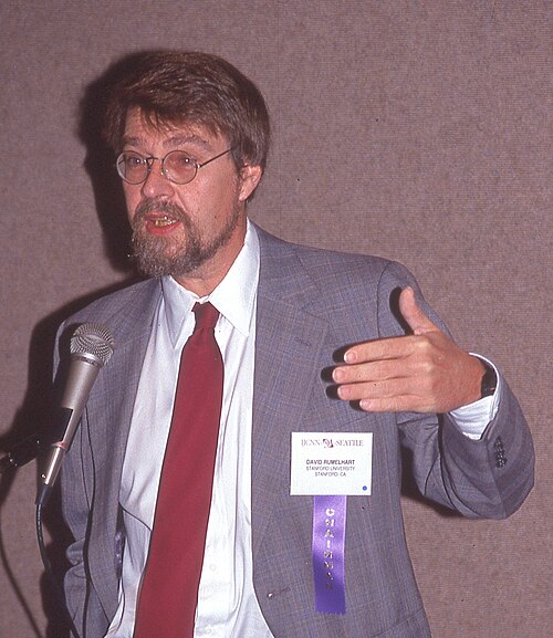
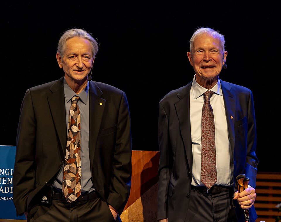
Rumelhart, Hinton and Williams show how to train many layers of weights by passing the error backwards.
1989–98
Yann LeCun’s team trains convolutional networks that read handwritten ZIP codes and bank checks.
2009
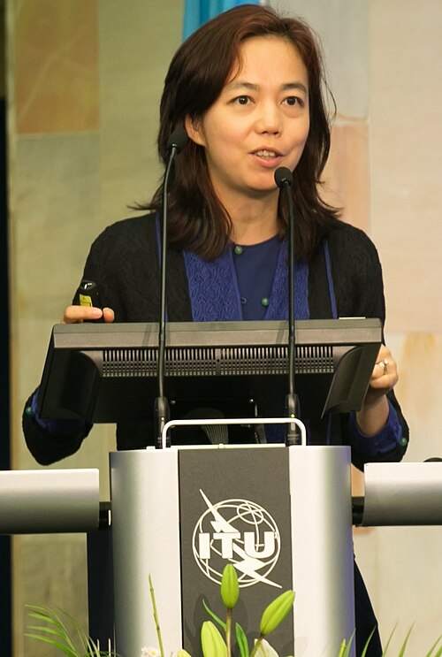
Fei-Fei Li’s team presents a database of millions of labelled photographs, a thousand times bigger than earlier sets.
2010
The GTX 580 arrives in November with 512 cores and a programming system that lets researchers use it for maths, not only games.
2012
All of it combined, on two GTX 580s, wins the ImageNet contest by a wide margin.
9BThe Arithmetic
In one line
The recipe was decades old. Big data and GPUs supplied the missing arithmetic: by my estimate about 200,000 times LeNet-5’s training operations, done in about five days.
about 4.7 × 10¹⁷
operations to train
Once a network like this is trained, people try to read it. One approach, the activation atlas (Carter and colleagues, 2019), lays out what thousands of neurons respond to in a single map. A more recent one extracted millions of interpretable features from a production language model (Anthropic, “Scaling Monosemanticity”, 2024). Both rest on the idea you just played with: the weights are learned, and what they have learned can be measured.
Paper: Krizhevsky, A., Sutskever, I. and Hinton, G. E. (2012), ImageNet Classification with Deep Convolutional Neural Networks, NeurIPS (NIPS) 25. All architecture, training and results figures are from this paper. Layer sizes and operation counts are my own arithmetic from the architecture it describes. Everything else is explanation of other people’s work, from my own study notes, with context from Wikipedia’s articles on AlexNet, LeNet, ImageNet and the GeForce 500 series.
Elephant and landscape photos (Wikimedia Commons): bathing elephant and river elephant by Basile Morin (CC BY-SA 4.0); walking away and savanna elephant by Daniel Case (CC BY-SA 4.0); mother and calf by JosepMGracia (CC BY-SA 4.0); tusker by Yathin S Krishnappa (CC BY-SA 3.0); trees on the savanna by Cosal (CC BY-SA 4.0); upland savanna by Gossipguy (CC BY-SA 3.0). Photos are scaled down for the page and otherwise unaltered.
People: Fei-Fei Li by ITU Pictures (CC BY 2.0); Ilya Sutskever by Eladkarmel (CC BY-SA 4.0); Hinton, LeCun and Rumelhart as credited on The godfathers of AI.
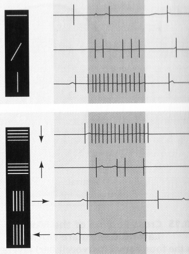
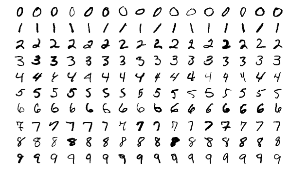
History photos (Wikimedia Commons unless noted): David Hubel by Joey cantod (CC BY-SA 4.0); Torsten Wiesel by Suawikicommons (CC BY-SA 4.0); neuron recordings diagram by Jimmierock (CC BY-SA 3.0); convolutional network diagram by Aphex34 (CC BY-SA 4.0); MNIST digits by Josef Steppan (CC BY-SA 4.0). Rosenblatt, the Mark I Perceptron, Rumelhart, LeCun and Hinton as credited on The godfathers of AI. Fei-Fei Li and Ilya Sutskever as listed above.
Not the paper’s own figures. The kernel grid, the learning demo and the embedding map are my own illustrations. They show the ideas; they are not AlexNet’s learned weights or outputs.