Rowan DasRotman Commerce Résumé

AI Projects

Project 1

The Perceptron: My First Project

The hello world of machine learning.

My first real machine learning project was a perceptron, one of the oldest learning machines there is. It has two weights and a bias. It adds up its inputs times their weights, and if the total is above zero it answers +1, otherwise −1. When it is wrong, it nudges every weight a little toward the right answer. That is all of it.

I gave it a small task, the logic AND gate: answer +1 only when both inputs are 1. Four examples, no libraries, about twenty lines of plain Python. It makes 10 mistakes in the first five passes over the data, then gets all four right and stops changing. The learned rule is 0.2·x₁ + 0.1·x₂ − 0.2 > 0, which is true only for (1, 1).

Language
Python, no libraries
Data
4 examples: the AND gate
Learning rate
0.1
Learned
weights [0.2, 0.1], bias −0.2
View the code on GitHubAmlan-Das/rowan-site · ai/perceptron/perceptron.py
Drag the slider (passes through the data) or press Play. Dark dots are the +1 example, hollow dots are −1. The line is where the score is exactly 0; the shaded side is where it answers +1. A red ring means that example is currently wrong.
Read the code
#Perceptron Steps

training_data = [([0,0],-1), ([0,1],-1), ([1,0],-1), ([1,1],1)]


weights = [0,0]
bias = 0        
learning_rate = 0.1

def activate(value):
    return 1 if value > 0 else -1


for epoch in range(20):
    for inputs, target in training_data:
        weighted_sum = sum(x*w for x, w in zip(inputs, weights)) + bias

        prediction = activate(weighted_sum)

        if prediction !=target:
            print(f"Epoch: {epoch}, Input: {inputs}, Target: {target}, Prediction: {prediction}")
            for i in range(len(weights)):
                weights[i] += (learning_rate*target*inputs[i])

            bias += learning_rate * target  

    for inputs, target in training_data:
        weighted_sum = sum(x*w for x, w in zip(inputs, weights)) + bias
        prediction = activate(weighted_sum)
        print(f"Input: {inputs}, Target: {target}, Prediction: {prediction}")
        print(f"Weights: {weights}, Bias: {bias}")


print(f"Final Weights: {weights}, Final Bias: {bias}")

This is the script exactly as I wrote it. The page above re-runs the same algorithm in the browser; its numbers match what the script prints.

Project 2

Cat or Dog: A Perceptron on Pixels

The same machine as Project 1, taken from 2 inputs to 1,024 pixels.

After the AND gate I wanted to see what the perceptron does on actual pictures. So I pointed it at images of cats and dogs: 300 for training and 70 for testing, which are small silhouette drawings rather than photographs. I wrote the whole thing myself in Python with NumPy, using torchvision only to load and shrink the images.

Each picture is squashed to 32 × 32 pixels, turned to grayscale and flattened into a list of 1,024 brightness values. The model is one weight per pixel plus a bias, all starting at zero. It adds up weight × brightness, answers 1 if the total is above 0 and 0 if not, and nudges the weights by learning rate × error × pixels whenever it is wrong. I trained it for 100 passes over the training folder, reshuffling the order each time, then loaded a separate test folder it had never seen. The code is unchanged below.

Data
300 train + 70 test drawings, half cats and half dogs
Input
32 × 32 grayscale = 1,024 numbers
Model
1,024 weights + 1 bias, rule w ← w + 0.01 · error · x
Training
100 epochs, shuffled
View the code on GitHubAmlan-Das/rowan-site · ai/catdog/catdog.py

What the Model Can and Cannot See

One weight per pixel means the model only knows how bright each fixed position is. It has no idea of ears, eyes or shape, and a cat shifted a few pixels lands on different weights. The training and test drawings are all variations of one icon per class, so a good score here says little about real photographs. That is the limit of this design, and it is what the AlexNet project below goes after: small shared filters that look for shapes anywhere in the picture.

The pipeline and the first update, run on one cat and one dog from my training folder, with the same steps as the code. ImageFolder numbers the folders alphabetically, so cat is label 0 and dog is label 1. The drawings are modified Font Awesome Free icons (Fonticons, Inc., CC BY 4.0), randomly rotated, resized, shifted and noised.

How the Accuracy Is Counted

The script counts a picture as correct when the model’s guess matches its label before that picture changes the weights, adds this up over all 100 epochs, and prints it divided by the total number of guesses. So it is a running training accuracy, not a score on unseen pictures. The script loads the 70 test drawings but its prediction loop is commented out, so I ran that same rule on the learned weights afterwards to get the test score shown here. Also, the printed correct divides by 1,000 although there are 100 epochs, so it reads 10 times too small: 0.0892 means an 89.2% average.

Read the code
import torchvision.transforms as transforms
from torchvision.datasets import ImageFolder
from PIL import Image
import numpy as np
import matplotlib.pyplot as plt

epoch_accuracies = []

weights_zeros=np.zeros(1024)
bias = 0 
learning_rate = 0.01


transform = transforms.Compose([
    transforms.Resize((32, 32)),
    transforms.ToTensor() 
])


dataset = ImageFolder(root="data/train", transform=transform)

print(dataset.class_to_idx)

correct = 0 
for epoch in range(100):
    image_tensore = np.random.permutation(len(dataset))

    for i in image_tensore:
        image_tensor, label = dataset[i]


        grey_image_transform = transforms.Grayscale(num_output_channels=1)

        grey_image= grey_image_transform(image_tensor)

        grey_flatten = grey_image.flatten()


        weidghted_sum = np.dot(weights_zeros, grey_flatten) + bias

        activation = 1 if weidghted_sum > 0 else 0


        error = label - activation  

        if label == activation:
            correct += 1

        #gonna have to multiply the error by the input values to get weight updates 

        result = np.multiply(error, grey_flatten) 


        #wnew weights = old weights + (learning rate * input * error)

        final = np.add(weights_zeros, result * learning_rate)
        weights_zeros = final
        bias = bias + (learning_rate * error)
        accuracy = correct / len(dataset) * 1000
    epoch_accuracies.append(accuracy)


    #transforms.ToPILImage()(grey_image).show()


accuracy = correct / (len(dataset)*1000)
print("Image Shape:", image_tensor.shape)
print("Class Label:", label)
print ("correct:", accuracy)

plt.plot(epoch_accuracies)
plt.title("Training Accuracy over Epochs")
plt.xlabel("Epochs")
plt.ylabel("Accuracy (%)")  
plt.grid(True)
plt.show()
plt.imshow(weights_zeros.reshape(32, 32), cmap="coolwarm")

plt.colorbar(label="Weight Value")
plt.title("Learned Pixel Weights")

plt.show()
imagefolder = ImageFolder(root="data/test", transform=transform)

test_dataset = ImageFolder(root="data/test", transform=transform)

print("Number of test images:", len(test_dataset))

'''
for tensor , dog in imagefolder: 
    grey_image_transform = transforms.Grayscale(num_output_channels=1)

    grey_image= grey_image_transform(tensor)

    grey_flatten = grey_image.flatten()

    weidghted_sum = np.dot(weights_zeros, grey_flatten) + bias

    activation = 1 if weidghted_sum > 0 else 0

    print("Predicted:", activation, "Actual:", dog)

    '''

This is the script exactly as I wrote it, including my variable names. It expects data/train and data/test folders with one sub-folder per class.

Research

The money, the people and the milestones behind modern AI.

Nobody really knows where AI is going, including the people building it. Most technologies show you their shape before they change anything. This one keeps surprising its own makers, and it has already become one of the forces behind almost everything happening right now: where the money goes, where the power plants go, what gets built, who gets hired, who gets nervous.

We are arranging the world around something we cannot predict. Maybe that is simply what living through a turning point feels like: plenty of headlines and very little explanation.

Now read the news.

Latest on the timeline

    On this pageTimelineDealsMachine learningGodfathers of AI

    The AI financing network. Who is paying whom in the AI buildout. Drag to turn it. See every deal ↓
    Two Decades of AI, 2005 to October 2026

    Two decades of AI, from the research that made it possible to the deals reshaping the economy today. Scroll sideways, and click any milestone to read the story.

    Dates and figures come from the linked sources, and some 2026 figures are from trade press and trackers. Latest entry: . New entries are added as big stories break.

    The AI Financing Network, Deal by Deal

    Who is paying whom in the AI buildout: the equity investments and purchase commitments between the AI labs, chipmakers, clouds, data center builders and power producers.

    Explore Every DealPick a company to see who pays whom, filter to the two-way pairs, or read all the deals as a table.Hands-on

    Pick a company to see its deals. The globe at the top of the page lights up the same selection.

    Equity investment Purchase commitment Technology collaboration Arrows point to where the value goes: an investment to the company that receives it, a purchase to the seller. A dotted line is a partnership with no money disclosed.
    Every deal as text
    DealTypeAmountWhat it is

    Drag the sphere to turn it. Amounts are as announced, and “up to” amounts are ceilings that may depend on milestones. Checked . Sources: .

    Project: How a Machine Learns

    I wanted to know what “learning” means in machine learning, below the headlines in the timeline above. So I built the smallest version that still learns: one layer of weights that reads handwritten digits, written in about thirty lines of Python with NumPy and trained on the MNIST data set. This section is the write-up of that project: what I built, how it works, what it achieved, where it fails, and what I took from it.

    The idea comes from Geoffrey Hinton’s lectures on the perceptron. The numbers live in a table called W, for weights, and the picture is a list called x. Everything below runs in your browser from the real weights my script produced, so each claim can be checked.

    Question
    Can a table of weights, nudged only when it is wrong, learn to read handwriting?
    Data
    MNIST: 60,000 training and 10,000 test digits, 28 × 28 pixels
    Model
    One layer: 10 rows × 784 weights = 7,840 numbers
    Training
    3 passes, 180,000 updates, rule: add x to the right row, subtract it from the guessed row
    Result
    88.1% on the 10,000 unseen test digits (87.2%, 85.5%, 88.1% after each pass)
    Limit
    One rigid template per digit: slide a digit sideways and it fails
    Sixty real handwritten digits from MNIST, the training set used below. The model is shown 60,000 of these.
    1. 1

      Look

      Turn the picture into x: one number per pixel, 1 where there is ink and 0 where there is not. A 28 by 28 picture becomes 784 ones and zeros.

    2. 2

      Score

      W has one row of weights for each digit. Add up that row’s weights wherever x has ink. That is the digit’s score. The biggest score is the guess.

    3. 3

      Check

      Compare the guess with the right answer, y. This is the only moment the model is told anything about the world.

    4. 4

      Correct

      Add x to the right row and subtract x from the guessed row. Do it for the next picture, and the next, tens of thousands of times.

    The write-up has six parts: how the data is represented, training, the update rule worked by hand, results and limits, where the idea is used, and the code. Each opens to a working demo.

    1Representation: What the Model SeesHow I turn a picture into a list of ones and zeros. Point at a pixel to read its number.Method
    What the Model Sees: A Picture Becomes X

    The model never sees a picture, only numbers. A scanner gives each of the 784 pixels a brightness from 0 to 255. Anything brighter than the cutoff counts as ink (1) and the rest as no ink (0). Pick a digit, move the cutoff, and point at a pixel to see its number.

    2Training, LiveA smaller version of the model you can train in the page. Watch blank templates sharpen.Demo
    Train It: Ten Digits, Thousands of Corrections

    The same rule, running live in your browser on ten digits drawn in a 5 by 7 grid, with some pixels flipped at random (marked with a red dot) so no two pictures are alike. Turn the messiness up and the digits get hard to read, even for you. Each template starts blank. Green means the pixel votes for that digit, red means it votes against.

    The templates are drawn from W. The percentage is measured on 400 messy pictures the model never trained on. With a lot of mess it plateaus: one layer of weights can only draw a straight line between digits.

    3The Update Rule, Worked by HandExactly what the two learning lines do, cell by cell, then a five-step walkthrough.Maths
    The Update, One Cell at a Time

    The two lines that do all the learning are W[y] += x and W[guess] -= x. Here they are on a 3 by 3 picture of a vertical bar (the middle column is inked, so x is 1 there and 0 everywhere else), with every cell's arithmetic shown.

    Squares are a drawing of vectors. The 3 × 3 picture is really 9 numbers in a row, and each row of W is another 9 numbers. “Add up the weights under the ink” is a dot product of two vectors. The grid only shows which number belongs to which pixel; the model works on the list.

    Watch It Learn: Three Shapes, Nine Pixels

    The same model shrunk until you can read every number. It has to tell a vertical bar, a horizontal bar and a diagonal apart. Press the button to step through five rounds of the loop: look, score, guess, check, fix.

    x

    The picture as a list: here 9 numbers, on a real image 784. Each is 1 (ink) or 0 (no ink). It is not a match against a template. It is only what the picture looks like.

    W

    The weights, a table with a row per digit and a column per pixel. A positive number says “ink here is evidence for this digit”. A negative one says “ink here is evidence against”. The model is nothing but this table.

    W @ x

    Multiply each row by x and add up. Because x is only ones and zeros, that is just the weights that sit under the ink, added together. One total per row: the scores.

    The update

    The right row gets x added, so the ink in this picture now counts for the right digit. The guessed row gets x subtracted, so it counts a little less for the wrong one. Right guess, and the two cancel.

    Weight Space: The Cone of Weights That Get Everything Right

    Here is another way to see the same learning. Treat the three weights as a point in 3D space. Each training example is a flat wall through the origin: weights on one side get it right, weights on the other get it wrong. The weights that get every example right fill a cone. Learning is just walking the point into the cone. Hinton draws this picture when he teaches the perceptron. Only three weights fit on screen, so this is 3 of the 784 you would have for a real digit.

    4Results and LimitsThe templates it learned from real handwriting, its test accuracy, and what breaks it.Results
    What It Learned From Real Handwriting

    The same rule, on 60,000 real handwritten digits from the MNIST data set, run as the Python below. Each picture is one row of W folded back into a 28 by 28 square. You can see a rough 0 ring, a 1 stroke and so on, with red where ink argues against the digit.

    Real output from the script below, run once with a fixed random seed. Accuracy is measured on the 10,000 test images, which are never used for training. It wobbles between passes because a perceptron keeps correcting itself rather than settling.

    Where It Stops: One Rigid Template per Digit

    Each digit gets a single template, and the winner is whichever template overlaps the ink the most. That only works while every digit is written the same way in the same place. Slide a real digit and watch the scores.

    Nothing about the digit changed, but its ink now lands on different weights, so the right template loses its lead. People write the same digit at different sizes, slants and positions, and one template cannot cover all of them. Hinton makes this point in his lectures: handwritten digits vary too much for “simple template matches of whole shapes.” The fix is more layers, which first learn small parts such as strokes and curves, then combine them.

    Uses the real learned weights above, on the 60 sample digits from the wall. Shifting moves the whole digit and fills the gap with blank pixels.

    5Where This Idea Shows UpMy model reading a ZIP code, and the real systems built on the same recipe.Context
    Where It Is Used

    The same recipe, a table of weights nudged whenever it is wrong, turns up in real products. Here is this page’s one-layer model reading a ZIP code.

    Digits are from the MNIST training set, read with the real weights from the script below. About one digit in eight comes out wrong, so nearly half of all five-digit ZIP codes would contain a mistake. The system LeCun’s team built for the US Postal Service in 1989 had an error rate of about 1%, and declined to answer on about 9% of digits instead of guessing.

    Reading handwriting

    Convolutional networks, which add layers to this idea, read US ZIP codes in the late 1980s. NCR’s check readers, in banks from 1996, were estimated to read about 20 million checks a day by 2001, around 10% of all checks in the US.

    Language

    Since 2002, perceptron training has been popular in natural language processing, for jobs like tagging each word in a sentence as a noun or verb and working out its grammatical structure.

    Scoring with weights

    Spam filters and ad-click predictors often start as a weight for each signal: a word, a website, a time of day. Add up the weights that apply and compare the total with a cutoff. That sum is W @ x.

    Today’s AI

    Image, speech and language models are the same loop at enormous scale: many layers and billions of weights, each guess compared with the answer and the weights adjusted. Calculus decides how much to change each one, instead of a flat plus or minus 1.

    Check and ZIP code figures are from Wikipedia’s article on LeNet, which cites LeCun and colleagues. The 2002 language result is Michael Collins’s, as described in Wikipedia’s article on the perceptron.

    6The CodeThe whole Python script, with a note on every part.Code
    The Code, Line by Line

    This is the whole program, unchanged. Each section is followed by notes: hover (or tap) a note and the line it explains lights up.

    What I Took From It

    Learning is repeated correction. The model is never told what a 7 looks like. It guesses, is told it was wrong, and moves the weights a little. After 60,000 pictures a 7-shaped pattern has built up in row 7.

    Training and testing are different pictures. Training runs over 60,000 images, three times, so 180,000 corrections. The 10,000 test images only measure the result, which is how you know it learned handwriting rather than memorised pictures.

    This is the smallest case. Modern models stack many layers of W, add a step that lets them bend the lines between classes, and replace “add or subtract x” with calculus that works out how much each weight caused the mistake. They also have billions of weights rather than 7,840. The loop is the same: score, compare, adjust.

    2012 Extension project: how AlexNet learned to see I took this one-layer model and asked what changes when it grows up: sliding kernels, vectorization, and the 2012 paper that made image recognition work. A second write-up, with the math and interactive demos.

    The Godfathers of AI

    Three researchers who kept working on neural networks through the long years when the approach was out of favour. In 2018 they shared the Turing Award, computing’s highest honour, and they are often called the godfathers of AI. Behind them stands a line of people going back to the 1950s.

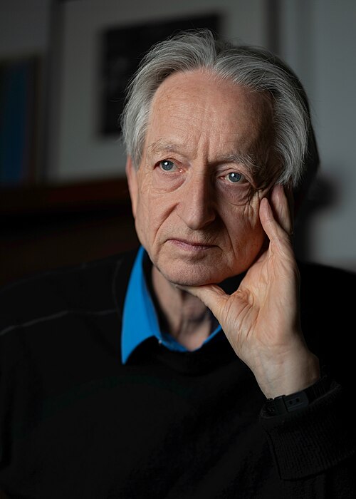
    Portrait photo of Geoffrey Hinton resting his chin on his hand

    Turing Award 2018 · Nobel Prize 2024

    Geoffrey Hinton

    Born 1947 · University of Toronto

    The one most often called the Godfather of AI. He worked on neural networks for decades and co-authored the 1986 paper that popularised backpropagation. With his students Alex Krizhevsky and Ilya Sutskever he built AlexNet, which won the 2012 ImageNet contest. He shared the 2024 Nobel Prize in Physics, and in 2023 he left Google to speak openly about the risks of AI.

    Portrait of Yann LeCun smiling, wearing dark-rimmed glasses and a navy jacket

    Turing Award 2018

    Yann LeCun

    Born 1960 · New York University

    Briefly a postdoc under Hinton. From 1988 he led LeNet, convolutional networks that read handwritten characters, and he co-created MNIST, the digits in the explainer above. A check-reading system he helped develop was widely deployed by NCR. He was Meta’s chief AI scientist before co-founding Advanced Machine Intelligence Labs in December 2025.

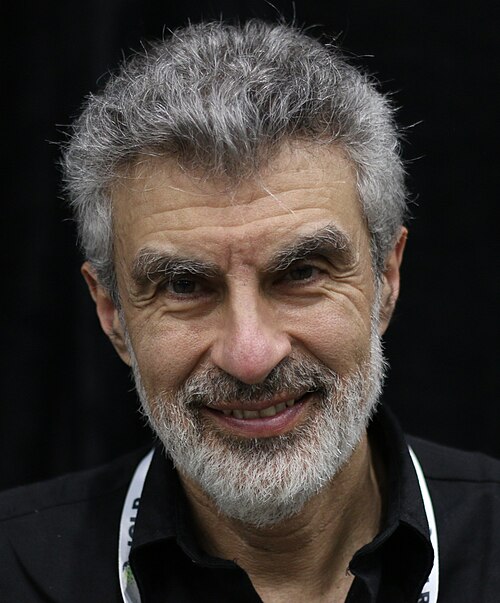
    Portrait of Yoshua Bengio with grey hair and a beard, smiling at the camera

    Turing Award 2018

    Yoshua Bengio

    Born 1964 · Université de Montréal

    He founded Mila, the Quebec AI institute, and was its scientific director until 2025. He is the most-cited computer scientist in the world, and in 2025 became the first AI researcher with more than a million Google Scholar citations. He now co-leads LawZero, a nonprofit.

    Where It All Started

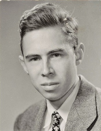
    Black and white portrait photo of Frank Rosenblatt as a young man in a jacket and tie

    1958

    Frank Rosenblatt

    1928–1971 · Psychologist, Cornell Aeronautical Laboratory

    Invented the perceptron, the learning rule in the explainer above: guess, and if the guess is wrong, nudge the weights toward the right answer and away from the wrong one. He first simulated it on an IBM 704 in 1957. In 1958 the New York Times headlined it “New Navy Device Learns By Doing.” He died in a boating accident in 1971, on his 43rd birthday.

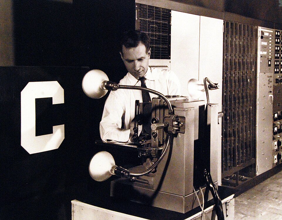
    The Mark I Perceptron

    Rosenblatt’s idea in hardware, built at Cornell Aeronautical Laboratory with Navy funding. Letters like the C in the photo were held in front of its photoelectric “eye”. The Navy’s own caption says that when it misidentified a letter, the trainer forced it to respond correctly, and that with a second typeface mixed in it was right 85 percent of the time.

    Black and white US Navy photo of a man at the Mark I Perceptron, with a large letter C lit up in front of the machine's photocell camera

    The People in Between

    Rosenblatt’s rule can only draw one straight line between classes. Most of what followed is the story of getting past that.

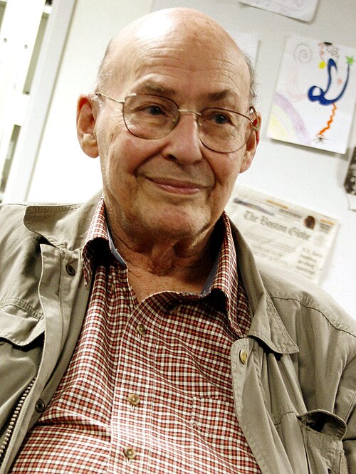
    Portrait of Marvin Minsky in a beige jacket and checked shirt

    1969

    Marvin Minsky

    1927–2016

    With Seymour Papert he wrote Perceptrons, which analysed what a single layer of weights cannot do. It is often credited with cooling interest in neural networks for years. The book was dedicated to Rosenblatt, who went to the same high school a year behind him.

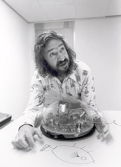
    Black and white portrait of Seymour Papert with long hair and a beard, resting his hands on a table beside a small domed robot

    1969

    Seymour Papert

    1928–2016

    Co-author of Perceptrons and an early AI pioneer at MIT. He later co-invented Logo, a programming language made for children.

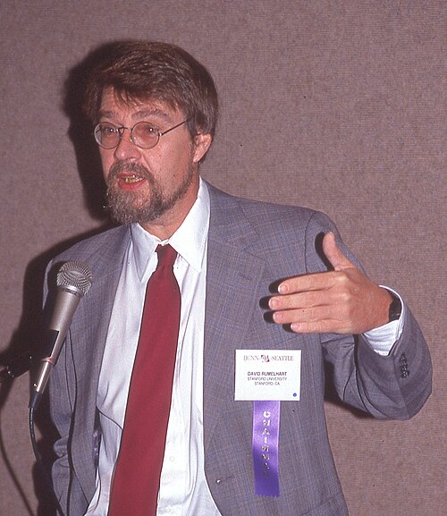
    Photo of David Rumelhart speaking into a microphone at a conference, wearing a grey jacket and red tie

    1986

    David Rumelhart

    1942–2011

    A psychologist who, with Hinton and Ronald Williams, published the paper that popularised backpropagation, a way to train many layers of weights instead of one. That is what gets past the straight-line limit.

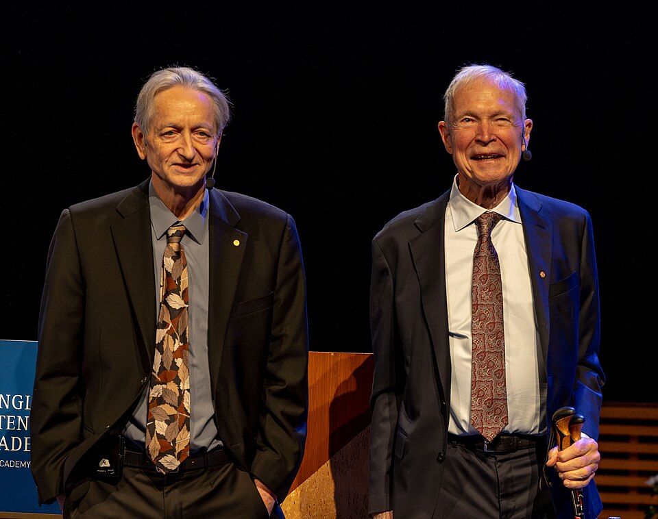
    Geoffrey Hinton and John Hopfield standing side by side on a dark stage during Nobel Prize week 2024

    2024

    Hinton and John Hopfield

    Nobel Prize in Physics

    Hopfield’s 1982 network helped revive interest in neural networks. In 2024 he and Hinton shared the Nobel Prize in Physics for foundational discoveries that enable machine learning with artificial neural networks.

    Photos from Wikimedia Commons, shown in black and white and otherwise unaltered: Hinton by Cmichel67 (CC BY-SA 4.0); LeCun by Jérémy Barande (CC BY-SA 2.0); Bengio by Xuthoria (CC BY-SA 4.0); Rosenblatt by Heinz Nixdorf MuseumsForum (CC BY-SA 4.0); Mark I Perceptron by the US Navy (public domain); Minsky by Sethwoodworth (CC BY 3.0); Papert by Matematicamente.it (CC BY-SA 3.0); Rumelhart by Rolf Kickuth (CC BY-SA 4.0); Hopfield and Hinton by Arthur Petron (CC BY-SA 4.0). Biographical details are from Wikipedia, the Navy’s caption for the Mark I photo, and the Nobel and Turing Award announcements as summarised there.